Tutorials

Two tutorials are provide here to acquaint the user with the MEA process model. The first is focused on property calculations, in terms of estimating the equilibrium partial pressure of CO₂ as a function of temperature and CO₂ loading. The second tutorial is focused on flowsheet simulation of the CO₂ absorption and solvent regeneration processes.

Predicting System VLE

1. Place the CCSI_MEAModel.bkp file and the supporting files ccsi.opt and ccsi10.dll in the same directory. Open the CCSI_MEAModel.bkp file. When prompted with the Column Sizing/Rating Detected box, select the Use Legacy Hydraulics option. If the Model Palette is not visible, it may be selected from the View tab at the top of the window. In the Model Palette, navigate to the Manipulators tab and then select Mult to create a multiplier block, which will be referred to by its default name B1. Double-click B1 and then set the multiplication factor to 1. Add an inlet stream to the block by clicking Material in the Model Palette, the red arrow on the inlet of B1, and then elsewhere in the flowsheet. Repeat the procedure for the outlet stream of B1. Name the inlet and outlet streams as IN and OUT, respectively.

   Note

   The streams may be renamed by double clicking the default name and typing the new name.

2. Double-click IN and configure it as follows:

   1. Select Temperature and Vapor Fraction as the Flash Type specifications.

   2. Temperature: 40°C.

   3. Vapor Fraction: 0.0001.

   4. Select Mass-flow in gm/hr as the composition basis. Set the values for H2O and MEA as 7 and 3 respectively.

1. In the left navigation pane, navigate to Model Analysis Tools ‣ Sensitivity and then click New. The new sensitivity block may be named “PCO2”. Under Manipulated variable in the Vary tab, select New, select Mole Flow as type, IN as stream, CO2 as component, and mol/hr as the units. Under Manipulated variable limits, specify 0.0005 and 0.03 as the lower and upper limits, respectively, and 10 as the number of points. Navigate to the Define tab and then create a new measured variable named PCO2. Under Edit selected variable, select Streams as the category, Stream-Prop as the type, IN as the stream, and PPCO2 as the prop set. Change the units to kPa. Navigate to the Tabulate tab and then click Fill Variables. Navigate to the Options tab and select the Do not execute base case option under Execution options.

3. Run the simulation by clicking the Run arrow or pressing F5. The results of the PCO2 sensitivity block should be consistent with what is shown in Table 1.

   Note

   All of the warnings that appear in the Control Panel while running the simulation may be ignored.

Table 1: Results of VLE Sensitivity Block

Row/ Case	Status	CO2 MOLEFLOW (MOL/HR)	PCO2 (KPA)
1	OK	0.0005	2.24E-5
2	OK	0.003778	0.00097
3	OK	0.007056	0.00363
4	OK	0.010333	0.00955
5	OK	0.013611	0.02339
6	OK	0.016889	0.06171
7	OK	0.020167	0.21295
8	OK	0.023444	1.47244
9	OK	0.026722	18.5729
10	OK	0.03	103.162

4. From this example, the vapor-liquid equilibrium (VLE) of the ternary MEA-H₂O-CO₂ system as a function of temperature and CO₂ loading may be determined for 30 wt% MEA. The CO₂ loading (mol CO₂ /mol MEA) may be calculated by multiplying the CO₂ molar flow by the molecular weight of MEA and dividing by the mass flow of MEA. For example:

\[\frac{\mathbf{0.0005\ mol\ }\mathbf{\text{CO}}_{\mathbf{2}}}{\mathbf{\text{hr}}}\mathbf{\times}\frac{\mathbf{61.08308\ g\ MEA}}{\mathbf{\text{mol MEA}}}\mathbf{\times}\frac{\mathbf{\text{hr}}}{\mathbf{3\ g\ MEA}}\mathbf{\approx 0.0102\ mol\ }\mathbf{\text{CO}}_{\mathbf{2}}\mathbf{/mol\ MEA}\]

Following this procedure and evaluating the sensitivity block for temperatures of 80 and 120°C, by changing the temperature of the stream IN and re-running the simulation, a plot similar to Figure 2 may be generated.

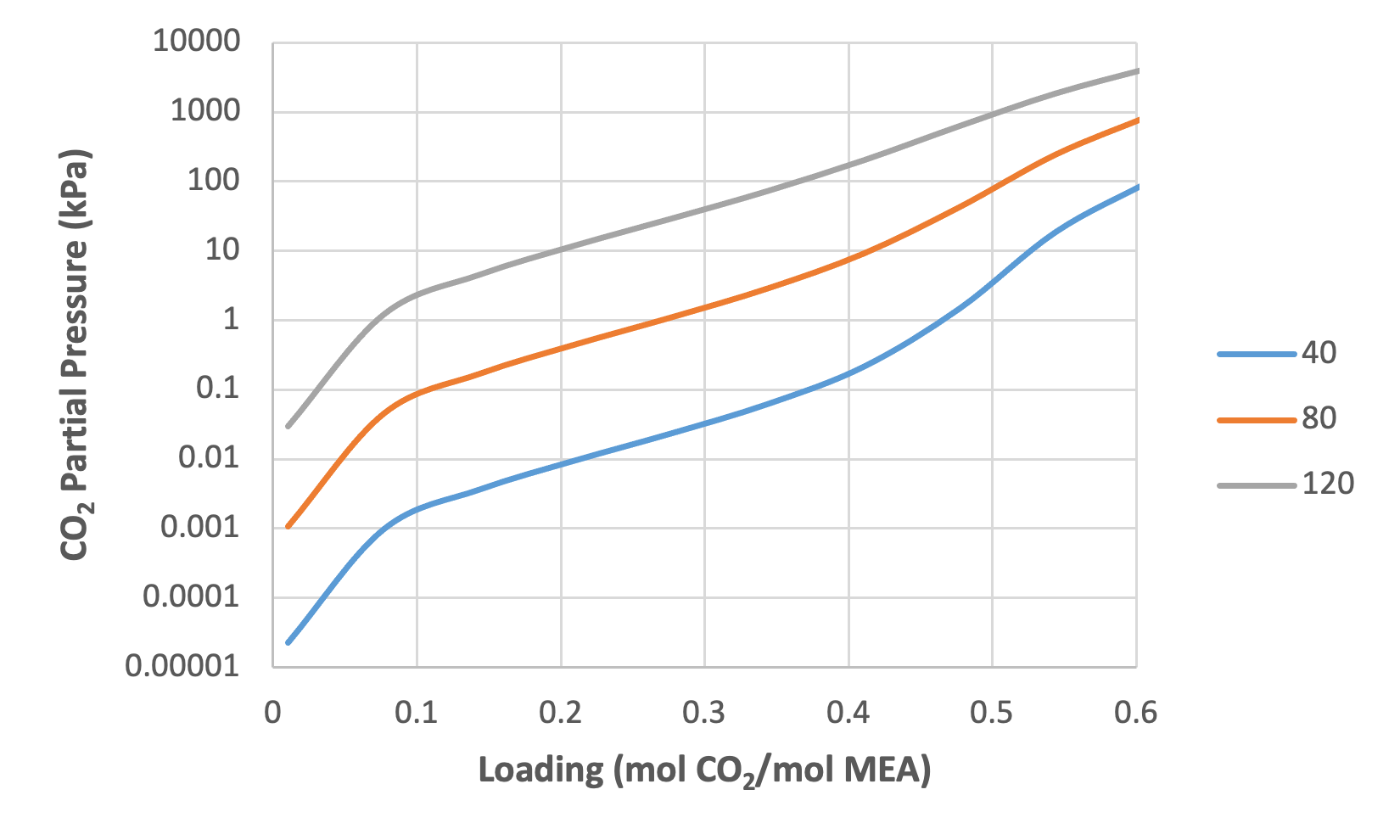
Figure 1: CO2 partial pressure as a function of loading and temperature (30 wt% MEA)

CO₂ Capture Process Simulation

The base case model that is set up in the file CCSI_MEAModel.bkp has operating variables and equipment configurations as specified in Table 2.

Table 2: Variables for Base Case Simulation

Variable	Value
ABSLEAN Stream (Absorber Solvent Inlet)
Temperature (°C)	40.97
Pressure (kPa)	245.94
Mass Flow (kg/hr)	6803.7
Component Mole Fractions
H2O	0.87457
CO2	0.01585
MEA	0.10958
GASIN Stream (Absorber Gas Inlet)
Temperature (°C)	42.48
Pressure (kPa)	108.82
Mass Flow (kg/hr)	2266.1
Component Mass Fractions
H2O	0.04623
CO2	0.17314
NO2	0.71165
O2	0.06898
Absorber
Intercooler #1 Flowrate (kg/hr)	7364.83
Intercooler #1 Return Temperature (°C)	40.13
Intercooler #2 Flowrate (kg/hr)	7421.57
Intercooler #2 Flowrate (°C)	43.32
Absorber Top Pressure (kPa)	108.82
Absorber Packing Diameter (m)	0.64135
Absorber Packing Height (ft)	60.7184
Regenerator
Inlet Temperature (°C)	104.81
Inlet Pressure (kPa)	183.87
Top Pressure (kPa)	183.7
Reboiler Duty (kW)	430.61
Packing Diameter (in)	23.25
Packing Height (ft)	39.6837

The variables described in Table 3 may be varied within reason, although abrupt changes in certain variables may results in failure of the simulation to converge. In the simulation provided in the example file, the variables for the ABSLEAN and GASIN streams can be located by double-clicking the respective streams. The variables for the absorber intercoolers can be located from the navigation pane by selecting Blocks ‣ ABSORBER ‣ Configuration ‣ Pumparounds, and the first and second intercoolers are referred to as P-1 and P-2, respectively. The top pressure of the absorber and regenerator can be located by double-clicking the ABSORBER and REGEN blocks and selecting the Pressure tab. Moreover, the reboiler duty for REGEN is located under the Configuration tab. The column packing diameters and height can be located by selecting Blocks ‣ ABSORBER or REGEN ‣ Sizing and Rating ‣ Packing Rating ‣ 1 ‣ Setup. The values of the regenerator inlet pressure and temperature are specified in the PUMP and EXCHANGE blocks, respectively.

Note

A sensitivity block, referred to as FLOW in the simulation, is used to set the flowrate of the inlet solvent stream, as the simulation will not automatically converge for such a low flow rate.

Next, the CO₂ capture process, which includes the absorber and regenerator columns, is evaluated for two sets of operating conditions.

1. Open the CCSI_MEAModel.bkp file. In the navigation pane, right-click Blocks, select Activate, right-click Streams, and then select Activate. Run the simulation.

   Note

   All streams and blocks have been deactivated to reduce the time required to obtain the results for the test in Section 2.2 Predicting System VLE. If block B1 and streams IN and OUT have already been created in the same file, they need to be deactivated by right-clicking them and selecting Deactivate before activating all streams with the aforementioned procedure.

5. In the flowsheet, right-click stream ABSRICH, select Results, and then select STRIPOUT from the drop-down arrow at the top of the right column. Ensure that the results obtained match those given in Table 3, noting that only selected rows are included in the table. The results shown in Table 3 were obtained from Aspen V10, and may vary slightly when using Aspen V11.

Table 3: Selected Stream Table Results

Mole Flow mol/hr	ABSRICH	STRIPOUT
H2O	260007	256376
CO2	0.344276	0.976410
MEA	8684.95	26272.89
MEA+	12184.17	3270.263
MEACOO-	11833.81	3152.68
HCO3-	350.36	117.58
N2	33.17	2.14E-16
O2	5.55	5.47E-18
Temperature C	52.01	120.94
Pressure kPa	108.82	183.7
Enthalpy J/kmol	-301829043	-281379385

6. Reinitialize the simulation by clicking Reset or pressing Shift+F5, and then selecting OK. In the navigation pane, navigate to Blocks ‣ Absorber ‣ Configuration ‣ Pumparounds ‣ P-1, and then change the flow rate to 3000 kg/hr. Navigate to P-2 and then change the flow rate to the same value.

7. Navigate to Model Analysis Tools and activate the FLOW sensitivity block, which is used to determine the CO₂ capture percentage in the absorber and the required reboiler duty for the stripper as a function of the lean solvent flowrate. Execute the model, navigate to the results of the sensitivity block, and verify that the results are similar to those shown in Figure 3; note that these results were generated using Aspen V10 and may be slightly different when running the model with Aspen V11.

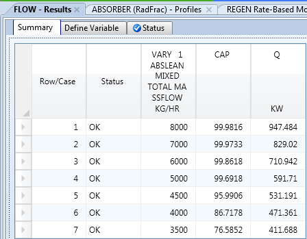
Figure 2: Results of the :guilabel:`FLOW` sensitivity block for the case study.

8. Navigate to Blocks ‣ Absorber ‣ Profiles and then highlight the columns labeled Vapor Temperature and Liquid Temperature. Under Plot on the Home tab, select Custom, and then verify that the resulting plot resembles Figure 4.

   Note

   These temperature profiles correspond to the last simulation executed (Case 8).

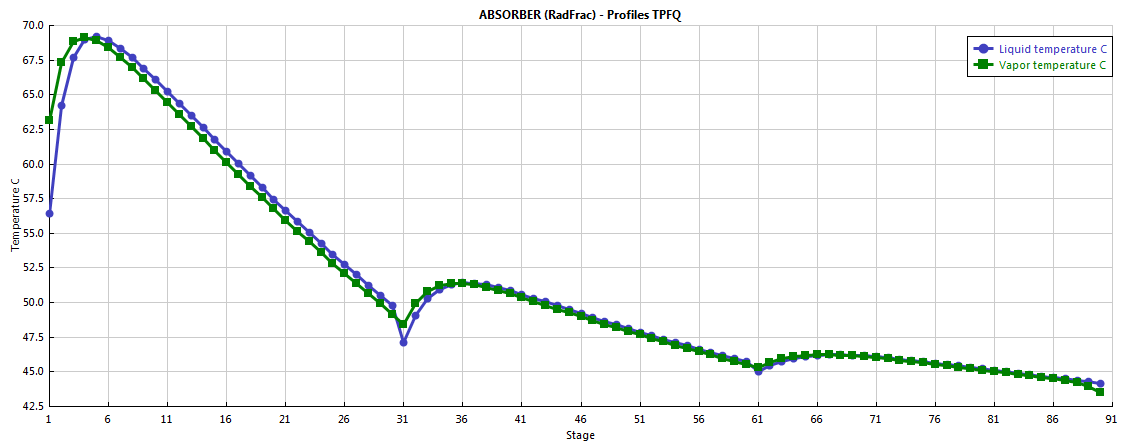
Figure 3: Absorber temperature profile for the case study.

9. Navigate to Blocks ‣ Regen ‣ Profiles and then repeat the procedure described in Step 5. Verify that the temperature profile resembles what is shown in Figure 4.

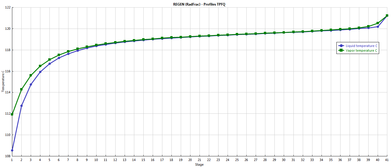
Figure 4: Regenerator temperature profile for the case study.